3D View Options Panel

Image-Pro with 3D Module only

When you view a sequence in 3D View mode, Image-Pro provides a panel to the right side of the image that includes a toolbar at the top and, below that, a set of options for each 3D View "node" added to the image.

All of the Add tools in the toolbar add nodes to the 3D view that contribute to the rendering of your volume.

Add Iso-surface/Volume measurement: Iso-surfaces provide a very quick, yet often sufficient, method for reconstructing polygonal surface models. By correlating transparency with the local orientation of the surface relative to the viewing direction, complex spatial structures can be understood much more easily.

Add 3D Colocalization: Adds 3D colocalization measurements with independent threshold levels.

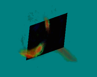
Add Ortho Slice: Clicking this button adds individual ortho slices to the ND projection. Ortho Slices are used to display a slice through the X, Y, or Z axis orientation in the 3D Viewer. Voxels on the plane of the slice will appear as a different color.

Each slice can have a different color outline. This can be useful for identifying slices on complex scenes with multiple elements (oblique, ortho slices). The visibility and the color of the outline can be set using the Outline control.

Add Oblique Slice: Oblique slices are used to display slices of the volume which are not precisely aligned with the X, Y, or Z axes.

Add External Object: External objects are iso-surface coordinate links that can be imported into the 3D Viewer.

Delete: Click this button to remove the selected node.

Expand/Collapse all nodes: Click the plus sign to expand the channels and nodes. Click the minus sign to collapse them.

The rest of the 3D View panel displays the rendering nodes that currently exist in your 3D visualization. The nodes and their specific set of controls can be one of the following:

C hannels
Ortho Slice
Oblique Slice
External Object
Volume Surface
Colocalization

Channels

All channels are loaded into an indexed color volume (The sequence is converted to a palette class using a palette containing the most popular colors in the sequence).. If the source image is a multi-channel image set, all monochrome channels are displayed in the list. The number of channels is not limited. Every channel has its own controls.

The channels node represents the visualization of the volume intensities. The drop-down box will only be enabled for multi-channel volumes, and controls the way that the channels are combined in the volume rendering. Clicking the drop-down arrow displays the following options:

• Max: Maximum Intensity Projection takes the value of the brightest voxel in the same straight line as used by the Blend option.

• Blend: Blending averages the values of the voxels in a straight line through the volume of the object.

• Min: Minimum Intensity Projection takes the value of the dimmest voxel in the same straight line as used by the Blend option.

Each channel of your volume will have a sub-node for the channel, with a name derived from the channel name (if the volume is a multi-channel set), the color component (of a color image), or “Gray” for monochrome images. Each channel or color component’s rendering can be adjusted using the controls provided.

The Show button hides or shows the selected element. Every node in the 3D View panel has this button, which lets you select which nodes are visible, and are included in the 3D rendering.

Every channel is shown using a palette that is scaled from 0 to 255 covering the whole dynamic range of the channel data. The All Channel Display controls will change Palette Spread and Opacity range on all channels.

The Blinking icon control activates the blinking mode of the channel.

The Palette can be one of the following:

• Wavelength allows you to display wavelength in nanometers.

• Color lets you select any color using the color picker.

• Palette allows you to select one of predefined palettes displaying the channel.

Activating the Histogram option allows you to set the Spread and Opaque levels on a volume histogram. Spread defines the start and end positions for palette spread and the Opaque control defines the range of intensities that are visible. The values outside the Opaque range are transparent. The Spread limits are controlled by the top controls and the Opaque limits are controlled by the bottom ones.

All-Channel Controls

The controls of the All-Channels node appy to all channels of the image. By default, every channel of the image is shown using a palette that is scaled from 0 to 255, covering the whole dynamic range of the channel data. The All channel Display controls allow you to change the palette Spread and Opacity range on all channels.

Spread: Defines the range of intensity values over which the image's palettes will be spread. In effect, this sets the baseline dynamic range for all channels of the image. It is initially applied to all channels of the image; however, it can be overridden at the channel level, if desired (see "Individual Channel Controls" below).

Best Fit: Click this option to have Image-Pro automatically detect and calculate the best-fit range values for every channel in the image and apply the widest best-fit range to the Spread spin boxes. This tool sets the high and low markers according to the highest and lowest pixel intensity values in the image. It sets the high and low levels such that the maximum dynamic range is achieved and no image data is lost.

Opaque: Defines the range of intensities that are visible. The values outside the Opaque range are transparent.

Reset: Click the Reset tool to reset the Spread and Opaque spin boxes to their default (full range) values.

Individual Channel Controls

Every channel has the following controls:

Show: The Show button toggles visibility of the given channel. If disabled, the associated channel will not be displayed in the image.

Blink: The Blink control activates the blinking mode for the channel. In Blink mode, the channel is repeatedly shown and then hidden.

Palette: The option you choose in the Palette pull-down list box defines the palette of colors that will be used by Image-Pro to display the range of pixel intensity values for the channel. You can choose from several pre-defined palette options, or you can choose one of the following customizable options.

Wavelength: Select this option to specify a wavelength, in nanometers, for displaying the channel. The palette for the specified wavelength is displayed above the palette pull-down list box.
Color: Select this option to specify a color, using color picker tool, for displaying the channel. The palette for the specified color is displayed above the palette pull-down list box.
Palette: Select this option to specify a predefined color palette pattern for displaying the channel. The palette for the specified pattern is displayed above the palette pull-down list box.
Selecting Custom palette allows creating user-defined color combinations:
- Palette points can be added by clicking on the histogram area. Clicking on an existing point makes the point active and allows color selection using the color-picker button which is located to the right of the histogram. The Position of palette points can be adjusted by clicking and dragging with the mouse. The Y position of the point defines the opacity of the color, the higher the position on the histogram, the higher the opacity. Hold the Ctrl key and Click on an existing point to delete it.
- Custom palettes can be saved to a file (pal3D format) and loaded (iqpal, pal3D) using the Save and Load buttons to the right of the palette drop down menu.
Histogram: Activating the Histogram option allows you to set the Spread and Opaque levels on a volume histogram. The Spread limits are controlled by the top controls and the Opaque limits are controlled by the bottom ones.

Spread from: Defines the range of intensity values over which the channel-specific palette colors should be spread. This overrides the spread specification defined by the All Channels Display spread control.

Opaque from: Defines the range of intensities that are visible for the channel-specific palette spread. The values outside the Opaque range are transparent. This overrides the spread defined by the All Channels Display spread control.

Best Fit: Click this option to have Image-Pro automatically detect and calculate the best-fit range values for the channel and apply those to the channel's Spread spin boxes. This tool sets the high and low markers according to the highest and lowest pixel intensity values in the image. It sets the high and low levels such that the maximum dynamic range is achieved, and no image data is lost.

Reset: Click the Reset tool to reset the Spread and Opaque spin boxes to their default (full range) values.

Ortho Slice

Ortho Slices are used to display a slice through the X, Y, or Z plane orientation in the 3D Viewer. Voxels on the plane of the slice will appear as a different color.

You can add multiple ortho slices. The following controls are displayed for each slice you add:

Orientation: Orientation selects one of three ortho slices, aligned with the X, Y or Z axis.

Type: Select the slice composition type: Opaque, Binary and Transparent. Binary means that voxels with non-zero alpha values are completely opaque and voxels with zero-alpha values are completely transparent.

Slice Number: Use the Slice Number slider to position the slice in the data volume. The slice is moved dynamically as the slider moves. You may also type a slice number in the spin box.

Handles: The Handles option controls visibility of the "dragger" associated with the ortho slice. The dragger can be used to drag the slice through the data volume. To use the dragger make sure the viewer is in selection mode (cursor is an arrow shape). Move the cursor onto the white cylinder, press the left mouse button, and drag to move the slice. You can also drag slices just by clicking and dragging the slice itself.

Clipping: Clipping enables the clipping plane associated with the slice. The clipping side can be either Front or Back. The clipping plane has no effect if the slice is not visible. Note that clipping affects other elements (slices, volume objects) added after the slice.

Smooth: The Smooth button switches on linear interpolation on the slice increasing the visible resolution.

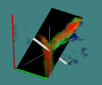
Oblique Slice

Oblique slices are used to display slices of the volume which are not precisely aligned with the X, Y, or Z axes.

You can add multiple oblique slices. The following controls are displayed for each slice you add:

Slice position: Use the Slice position slider to position the slice in the data volume. The slice is moved dynamically as the slider moves. You may also type a slice number in the spin box.

Alpha angle and Beta angle: These sliders allow you to change the orientation of the slice.

Smooth: The Smooth button switches on linear interpolation on the slice increasing the visible resolution.

External Object

External objects are Iso-surface coordinate links that can be imported into the 3D Viewer. Multiple external objects can be added clicking the Add External Object button. The objects can be loaded from Open Inventor (*.iv), VRML (*.wrl) or STL files.

The loaded external object can be edited by clicking on it in Select mode:

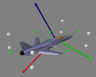
Using the "dragger" the object can be scaled, rotated and moved. Tip: holding down Ctrl-Shift keys allows adjusting the dimensions independently.

Clicking the object again will switch off visibility of the draggers.

Volume Surface/Iso-Surface

Automatic segmentation of 3D objects can be done using one of 2 different tools:

- Add Volume Measurements

- Add Iso-Surface

The Add Iso-Surface segmentation is based on iso-surface, which is generated using the Marching cubes algorithm with consequent labeling of mesh triangles (we will call it "Iso-Surface segmentation"). The Add Volume Measurements uses segmentation creating objects directly based on voxel connectivity data, without generation of iso-surfaces (we will call it "Direct Volume Segmentation").

Both methods have their advantages, which will be compared here:

Advantages of Direct Volume Segmentation over Iso-Surface segmentation:

Lower memory usage. Since no iso-surface is generated, the memory requirements for direct segmentation is much lower than for the iso-surface segmentation, which allows segmenting larger volumes.
Faster segmentation. The segmentation is applied to a 3D volume directly, the algorithm uses a single pass labeling, which significantly speeds up the segmentation, up to 100 times on complex volumes.
Holes handling. Direct segmentation algorithm handles holes according to the Fill Holes option, which allows user to decide if they want to include or exclude the holes from segmented objects. Generated Hole measurements (Hole Count, Hole Volume and Hole Volume Ratio) are available only for directly segmented objects. The iso-surface segmentation handles holes differently, the holes are always included into the surface object measurements, no Hole measurements are generated.

Drawbacks of Direct Volume Segmentation over Iso-Surface segmentation:

When Direct Volume Segmentation is used no iso-surface is generated, which leads to some drawbacks.

Saving segmented objects. The segmented objects cannot be saved as 3D models to IV, WRL or STL files. If you need to have a 3D model file, you should use iso-surtface segmentation.
Derived measurements. Derived measurements that use volume objects, such as Distance between surfaces, Point to Surface are not available for Direct Volume Segmentation.
Pixelated visualization. Visualization of 3D objects are done using shader rendering on GPU, so it misses some smoothing effects of triangular mesh iso-surface rendering. You can change material appearance of segmented objects using Pseudo Surface tools, such as pseudo-surface material or using the Voxelize option in the Interpolation drop-down. If object visualization is important, you should use the iso-surface segmentation.
Clipping of channels and segmented objects. Clipping planes created by ortho and oblique slices can clip iso-surface objects and volume independently, depending on the position of the slice relatively to the iso-surface element in the options tree, so volume can be clipped, but the surface not. With Direct Volume Segmentation both Volume Channels and Segmented objects are clipped in the same manner.

Click the Add Volume Measurements button to initiate a segmentation and (if desired) count operation to have Image-Pro auto-detect objects of interest and add Iso-surfaces identifying them in the image. Note, that this action is the same as clicking the Count button on the 3D Measure tab. When you click it, the Add Volume Measurements dialog box is displayed.

The segmentation with default options has advantages on memory consumption and speed over iso-surface segmentation, and if you want to get even better performance measuring the volume, click on the Advanced button to show the Fast mode options dialog box. This dialog box has the following options:

Activate pseudo surface: The Activate pseudo surface options check-box makes the best visualization options for direct segmentation surfaces active automatically. When this option is on, the volume visualization is automatically switches to the Pseudo Surface mode.

Create Preview volume: The option Create Preview volume defines creation of the visualization volume for threshold adjustment preview. You can switch this option off to save RAM, in that case threshold preview will be generated on the original volume channel and may look slightly different from the segmented volume as they may have different sub-sampling and filter options.

Create segmentation volume: When the Create segmentation volume is on, the segmented objects are shown in different colors on the volume. If user just want to have measurements and the visualization is not important, this option can be switched off to save more RAM. Note, that all measurements will still be generated properly and object volume boxes will be displayed for selected objects. When this option is off user can show equivalent spheres instead of the proper outline by activating the Show object equivalent spheres option, spheres display takes less RAM then the segmentation volume and can be used to handle large volumes when Create preview volume and Create segmentation volume options are off.

For more information on using this dialog box to define initial 3D segmentation parameters, and to perform a 'count' of auto-detected 3D objects, click here. The following controls are displayed in the 3D View Options Panel for each volume measurement definition you add:

Histogram Display: You can use the histogram display to adjust the segmentation threshold levels as you review the effects of your changes on the resulting object detection in the image. The thresholds can be adjusted by clicking and dragging the start or end of the threshold range on the histogram, or by editing the upper and lower limits in the From and To controls. Once you are satisfied with the resulting object detection, you can then execute the count by activating the Count check box.

Color: The color setting is useful for visualizing the results of segmentation prior to activating the Count check box. When the Count option is turned off, the color of Iso-surface can be adjusted in the Color drop-down. Note that when Count is on, the colors of individual objects are controlled by the Coloring parameter of the 3D Measurement options panel. When Coloring is set to Iso-surface the segmented objects have the color of Iso-surface, when the Coloring is set to Random, then the color of every segmented object is selected randomly, but the transparency is taken from the Iso-surface.

There are different methods of displaying semi-transparent objects that can be selected pressing the "Q" key. Some methods produce better quality, but may slow down the rendering. Additional color controls can be accessed by double-clicking on an object in the image. For example, object 1:9 is selected in the example below.

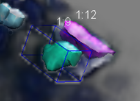
If you were to double-click on it, you would access a dialog box that allows you to modify its appearance attributes. Click here for more information.

Options: Clicking the Options button allows you to edit surface parameters, such as Sub sampling, Filter, and Threshold Type. These are described below.

Sub sampling: Use the controls in the sub-sampling group to limit processing to a sub-sample of pixels. When X, Y, and Z equal "1," then every pixel of the image is processed. A subsample of "2" causes Image-Pro to process only every other column (X=2) or row (Y=2) or stack (Z=2) of pixel data. If you set an axis's value to "3," only every third column, row or stack is processed, and so on. Use sub-sampling for large volumes to improve the speed of the rendering function. Selecting the Auto checkbox activates Image-Pro's automatic sub-sampling mode. In this mode, the sub-sampling is calculated based on the size of the image. This provides faster loading and rendering of volume images. By default this option is on. Advanced users can switch this option off and set sub-sampling manually.
Filter: Filters can be used to smooth the surface. A filter can be selected from the following list: None, LoPass 3x3x3, LoPass 5x5x5, LoPass 7x7x7, LoPass 9x9x9, Gauss 5x5x5, Gauss 7x7x7, Gauss 9x9x9.
Threshold type: This will show "Current" by default. If you want to reset the threshold, you can change it to "Auto Bright," "Auto Dark," or "Manual".
Close Edges: Select this option to have Image-Pro close the surfaces of the objects where they touch the bounding box of the volume. When Close Edges is turned on, the surface is closed on the sides that touch edges regardless their intensity value. (The edges must be closed to measure volumes.)
Activating Auto Split option will use watershed algorithm to split objects after segmentation. The option can be used to automatically split touching volumes. When the Ridge size option is active, only narrow junctions with diameter below the given size are split. Note that the split is also applied after adjusting the threshold levels of the segmentation.
Fill Holes option is on, the holes are included into the measurements of the segmented objects.
If Clean borders is on selected the objects that touch the bounding box of the volume are excluded from the analyzing.

Using the Add Iso-Surface tool, the Add Iso-Surface dialog box is displayed allowing you to create the iso-surface based segmentation.

The Precision control defines whether surface outlines of 3D object are created with Sub-voxel or Voxel granularity. The default option is Sub-voxel. This option allows creating smooth surface outlines that can be created in sub-voxel space and the position of this outline depends how close the threshold value is to the intensity value of the voxel.

When the Voxel option is active the surface outlines and all volumetric measurements are build from voxel cubes. Voxels with intensity above or equal the threshold level are completely included into the object.

Click the Ok button add the iso-surface. The new node's controls appear in the 3D View Options panel.

Among the node's controls are the Export and Import tools:

Export: The visible volume measurement objects can be exported to an IV or STL file clicking the Export button.

Import: If desired, you can import volume objects using the Import button. This option can be used, for example, when you have segmented objects on one channel and wants to measure intensities within these outlines on another channel.

Colocalization

Colocalization measurements with independent threshold levels can be added using the Add 3D Colocalization Measurements and Add 3D Colocalization Iso-Surface buttons. Both actions will create colocalization measurements, the difference is the same as for volume measurements and iso-surface, the first one creates colocalization using direct volume segmentation and the second - using iso-surface segmentation. Colocalization measurements are similar to volume measurements. They provide all measurement parameters available for a volume object and also include specific colocalization measurements.

Clicking the Colocalization tool in the 3D View Options panel displays the Add Colocalization dialog box where you can define the colocalization pair and also the initial auto-threshold method. The default method is Auto-Bright. Click the Ok button to create a new Colocalization measurement and open the Colocalization panel with colocalization scatterplot and the table with colocalization parameters. The scatterplot window shows the intensity distribution for two channels.

Colocalization thresholds can be adjusted for each channel independently using Channel 1 and Channel 2 numeric controls, dragging threshold levels on histogram or clicking on scatterplot. The colocalization objects and measures are updated automatically.

It is also possible to use Free ROI tools to define colocalization areas on the scatterplot, the colocalization objects get updated after creation or adjusting of ROIs. Note, that adjusting thresholds on histogram switches colocalization mode to “Thresholds”.

3D view may include multiple colocalization pairs. The colocalization panel shows results for the active colocalization pair. To activate the pair click the Colocalization button. When the Count option is active, colocalization measurements can be reported for every object. To add colocalization to the list of selected measurements, click the Add Measures button. The measures will be added to the list and shown in the data table.