Intensity Calibration
When you select the Int.Cal. option from the Calibration group, the Intensity Calibration dialog box appears in the details panel. This dialog box allows you to view, create, and edit intensity calibrations and apply them to your images.
Toolbar Tools
The dialog box's toolbar includes the following tools:
Apply: Applies the current calibration to the active image.
New: Use this tool to create new intensity calibrations.
Load: Allows you to load a calibration definition from afile. Loads calibration(s) from *IQI files.
Save: Use this tool to save the current calibration to a file.
List reference calibration only: When activated only calibrations with a reference flag are included in the list.
Reference calibration: This control shows whether the current calibration has reference flag. Clicking the button changes the Reference flag of the current calibration. Note that only Reference calibrations are persistent from one application session to the next.
Delete: Use this tool to delete the current calibration (calibration can be deleted if it is not assigned to any of opened images). Optionally, click on the drop-down menu to access the Delete All button.
Reset: Use this tool to reset the current calibration to default values.
Edit: Click to show/hide the options for editing intensity calibrations. See "Options/Edit Calibration" below for more information.
Dialog Box Tools
From within the Intensity Calibration dialog box, you can apply an open set of calibrations to the image, or you can create a new set of calibrations by clicking the New button and entering your calibration values in Edit mode.
In the list-box on top of the dialog box (Calibration Name) select the set of calibration values you want to apply to the image. If you want to use the gray levels, select (none). Any calibration sets that were loaded or created since the application window was last opened, will be listed in this list box.
You will not be able to enter calibration values until a name other than (none) has been selected in the Name list box. If (none) is the only set listed, you can create a set by clicking the New button and specifying its calibration values.
By default, the Application will assign the name "Intensity Cal 0" to a new calibration set; however, you may change this to a more descriptive name if you'd like.
New: Click this button to create a new set of calibration values. When this button is clicked, the Application will place the "Intensity Cal 0" name in the Name list box (the 0 digit may be incremented to make the set name unique) and show the calibration curve.
Units: Type the name of your unit in this field (e.g., density, degrees, disbursement). This name will appear when the Application reports intensity data.
Abbreviation: The short name of the units (as OD, ng etc.).
Log scale X and Y controls toggle logarithmic scale along the corresponded axis on the chart.
Calibration curve is shown in red color and the sample points used to create the calibration are shown as blue stars. The X axis represents the input values, which are in gray values and the Y axis is the Output values in calibrated units.
R-square: shows the goodness of fit of the calibration curve to the sample points. The range of the value is from 0 to 1. The perfect fit corresponds to 1.0 value.
Options/Edit Calibration
When you click on the Options/Edit Calibration button at the bottom of the Intensity Calibration dialog box, the Options/Edit Calibration section of the dialog box is displayed. Use the controls in this dialog box to modify the currently selected intensity calibration. The Options/Edit controls are organized into three groups:
Data Table Toolbar
The toolbar of the Options/Edit Calibration section of the Intensity Calibration dialog box provides the following tools:
Load: Use this tool to load calibration points and outlines from a file
Save: Use this tool to save the current calibration points and outlines to a file
Picker: Pick the intensity value from Image
Insert calibration point: Click this to insert a new point after the selected row. The Input and Output values of the new points are calculated as the average from the previous and next points.
Step Template Wizard: Click this tool to run the Step Tablet Wizard
Show: Show sample areas overlay
Edit Mode: Activate Edit
mode for sample areas.
Data Table Options
In the data table area, you will see the following controls.
Type - The context of the table depends on the type of the intensity calibration, which can be one of the following:
- "Free form" - The calibration is calculated from a number of user-defined sample points that are fit to a polynomial. The type of polynomial and its order are set via Sample Points and Fitting Mode.
- "Optical Density Standard" - The calibration is defined by two intensity values: Black Level = the intensity read by the acquisition device for totally opaque samples. Incident Level = the intensity read by the acquisition device for totally transparent regions. The calibration response curve is calculated using the standard optical density formula, which assumes that light decays exponentially as it goes through light- transmitting material: OD(x,y) = -log ((I(x,y) - BL) / (IL - BL)), where BL and IL are the Black Level and the Incident Level respectively, and I(x,y) is the intensity at location x,y.
- "LUT" - the calibration is not calculated, but it is defined by a LUT given by the client.
- "Neutral" - A neutral
calibration where calibrated values are mapped directly to gray levels.
This calibration is useful to associate a calibration unit name with an
image.
Fitting - This control is available only when the selected Type is "Free form". The following Fitting types are available:
- "Linear" - piecewise linear interpolation
- "Polynomial, order 1" - polynomial fit first order (regression line)
- "Polynomial, order 2" - polynomial fit second order
- "Polynomial, order 3" - polynomial fit third order
- "Lagrange, order 1" - piecewise linear interpolation first order (same as 0)
- "Lagrange, order 2" - piecewise interpolation second order
- "Lagrange, order 3" - piecewise interpolation third order
- "Optical Density" - fitting to an optical density function of the form y = -log10(ax + b)
- "Exponent, order n" - fitting to a function of the form y = exp(P(x)), where P(x) is a polynomial of degree 1, 2 or 3. Degree 1 is typically the most useful one.
- "Logarithm, order n" - fitting to a function of
the form y = -log(P(x)), where
P(x) is a polynomial of degree 1, 2 or 3. Degree 1 is typically the most
useful one.
Monotonic - This control forces the calibration LUT to be monotonic. In most cases, the calibration LUT must be monotonic (i.e. there are no two gray levels with the same calibrated value, such that these two levels are separated by other gray levels with different calibrated values.). This option can be used to force the calibration to be monotonic.
Positive - This control forces the calibration response LUT to be positive (zero values allowed). When the LUT is calculated from calibration points, there is a possibility that the curve described by the LUT will have negative values. In real-life situations, negative values are not possible. This option guaranties that the LUT is clipped by the y=0 axis.
Number of samples - defines
the length of calibration LUT.
Data Table
In the Free form mode the table contains 4 columns:
The data table height can be adjusted by dragging the separator between the graph and the table. The data table contains the sample points used for creating the calibration.
Input and Output values can be changed manually editing the cell value in the table. The calibration curve is automatically updated after the change. The Input value can also be picked directly from the image selecting the corresponded table row and clicking the Image button or by just clicking on the corresponded cell in the Image column. The following prompt will be displayed: "Click on image to pick the value".
Select a shape (Circle or Rectangle) and size/diameter for the picker tool. Clicking on the image will create a new sample area and the average intensity from the area will be used as the input value for the sample point. When the sample point is associated with area on the image the center coordinates of the area are displayed in the Image column.
The visibility of the created sample areas is controlled by the Show sample areas overlay button. Activating the Edit mode allows moving and resizing the existing areas using the following controls:
- Left-click to select.
- Shift-left-click to add to selected group.
- Left-click and drag net to select a group of objects.
- Left-click and drag hand to move selected object(s).
- Left-click and drag handle to edit object.
The calibration curve is automatically updated after the editing of the sample areas.
Step Tablet Wizard
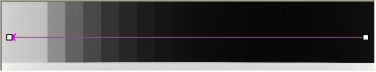
Intensity calibration can be created from a step-tablet image with known optical density values using the Step Tablet Wizard. Clicking the Step Tablet Wizard tool button launches the wizard prompting you to draw a line from center of the first to the center of the last step-tablet:
When the line is created the bands on the step-tablet image are automatically detected and labeled:
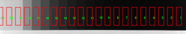
The user then has to add the correct Output values for every Input value in the table.
Tip: You can create a file with Output values for certain types of step-tablets and use it with multiple images using the Load and Save buttons.